Future of LLMs might not be Autoregressive
Intro to the world of block diffusion


If you’ve been paying attention to the language model space over the past few years, one fact is impossible to ignore: we live in an autoregressive world. From GPT-5 to Qwen3 or Llama, every major lab has followed the same next token prediction pipeline, left to right, one at a time. It’s a paradigm so dominant that it’s become synonymous with “language modelling” itself.
What if next-token prediction is just an artifact of how we built these systems?
What if a “language model” is something more than a next token predictor?
A different approach is quietly gaining traction: diffusion language models. Companies like Google, Inception Labs, and several research labs are publishing an increasing number of papers exploring this direction. In 2024-2025 alone, we’ve seen models like LLaDA, Dream 7B, and Block Diffusion demonstrate comparable performance to autoregressive approaches. Unlike the continuous diffusion that powers image/video generators such as Stable Diffusion and Veo3, these are discrete diffusion models built specifically for text. This is the approach running inside Google’s Gemini Diffusion and Mercury from Inception Labs.
This post is not a ground-up tutorial on autoregression or diffusion. If you want those:
For diffusion basics: https://lilianweng.github.io/posts/2021-07-11-diffusion-models/
For language diffusion in general: https://spacehunterinf.github.io/blog/2025/diffusion-language-models/
For autoregressive LMs: https://jalammar.github.io/illustrated-transformer/
We’ll move in three steps. First, we’ll quickly recap how standard autoregressive models work. Second, we’ll look at how diffusion language models approach the same problem differently. Finally, we’ll talk about the different diffusion model approaches.
Part 1: The Autoregressive Paradigm
How Autoregressive Models Work
Let’s start with what currently powers virtually every production LLM. An autoregressive language model factors the probability of a sequence as a product of conditional probabilities:
In plain English: predict each token given all previous tokens, one at a time, left-to-right.
Architecture: Typically a decoder-only Transformer with:
Causal attention mask (token i only sees tokens <i).
Position embeddings to encode order.
A final softmax layer producing
\(p_θ(x_i∣x<i) \)over the vocabulary.
Training: The model learns to predict the next token using the actual previous tokens from the training data, optimized with cross-entropy loss
You feed in the ground-truth prefix x_{<i} and train the model to predict x_i.
Inference: Sequential sampling:
Start with a prompt or BOS token.
Sample
\(x_i∼p_θ(⋅∣x_{<i}) \)Append x_i to the sequence.
Repeat until EOS or max length.
Pros of Autoregressive Models
Conceptually natural: Matches how we read and write language sequentially.
Efficient inference (with KV caching): Each new token requires only incremental computation.
Strong empirical performance: GPT-5, Claude, Llama all use this approach.
Easy to train: Stable gradients, well-understood optimization.
Cons of Autoregressive Models
Unidirectional: Only sees left context, not future tokens.
Sequential generation: Limited parallelism during decoding.
Commitment problem: Must decide on early tokens before seeing what comes later.
Reversal asymmetries: Autoregressive LMs have been known to memorize facts like “A is B” without generalizing to “B is A”, this is called the reversal curse.
Constraint enforcement is tricky: Autoregressive models generate text one token at a time, making it hard to enforce rules that apply to the whole sequence (like “include these exact phrases”).
This is particularly interesting because if you want an AR model to generate text that satisfies some global constraint, you typically need:
Careful prompting
Rejection sampling (wasteful)
Guided decoding (complex)
Or fine-tuning specifically for that constraint
Wouldn’t it be nice if the model could see the entire sequence context when making decisions about each token? That’s where diffusion comes in.
Part 2: Why Diffusion Conquered Images
Before we get to language, let’s understand why diffusion works so well for images.
Continuous Diffusion in 60 Seconds
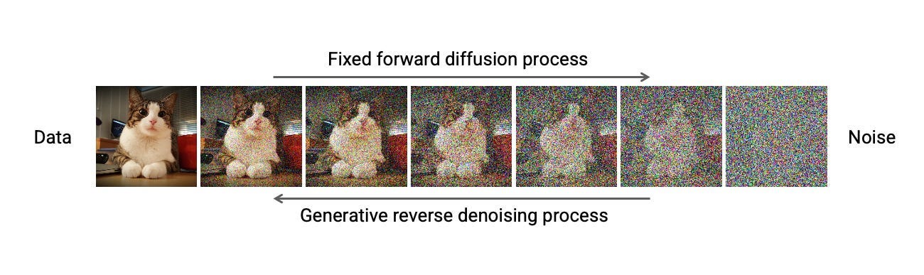
The classic diffusion story (DDPM, Stable Diffusion):
Forward process (noising):
Start with clean data x_0 (an image).
Gradually add Gaussian noise over timesteps t=1,2,…,T.
At inference, start from x_T and iteratively denoise:
\(x_{t−1}∼p_θ(x_{t−1}∣x_t)\)End with pure noise
\(x_T∼N(0,I)\)
Mathematically:
Reverse process (denoising):
Train a neural network ϵ_θ(x_t,t) to predict the noise added at step t.
After T steps, you get a clean sample x_0.
Why this works for images:
Pixels are continuous (RGB values are floats).
Adding Gaussian noise to floats is natural and smooth.
Small noise perturbations create small perceptual changes.
Iterative refinement aligns with multi-scale image structure.
The Discrete Problem: Why Text Is Different
Text is fundamentally discrete. Each token is an integer index into a vocabulary.
Images: You can have pixel value 127.4 or 127.5 - both are “valid” pixel values.
Text: There’s no “state between ‘cat’ and ‘dog’” - tokens are atomic.
If you naively apply continuous diffusion to text:
Embed tokens into continuous vectors.
Add Gaussian noise in embedding space.
Denoise to get refined embeddings.
Round back to discrete tokens via argmax or sampling.
This was tried in early works like Diffusion-LM (2022) and GENIE (2022). The problems:
Rounding is lossy and unstable: Small changes in embedding space can cause large semantic shifts.
Embedding space is not uniform: The discrete token distribution doesn’t match the continuous noise distribution.
Long-range coherence suffers: Each rounding decision compounds errors.
So while continuous diffusion exploded in computer vision, autoregressive models continued to dominate NLP.
The community needed a fundamentally different approach: discrete diffusion.
Discrete Diffusion: The BERT Connection (And Why It’s Not BERT)
Here’s where things get interesting. If you squint, discrete diffusion looks a lot like BERT. Both mask tokens. Both predict what’s missing. But the similarity is superficial like comparing a bicycle to a Tesla because both have wheels.
BERT-Style Masking: The Fixed-Ratio Autoencoder
BERT’s masked-language-model objective looks similar in principle to what discrete diffusion models do. During pre-training, BERT:
Randomly selects 15% of token positions in the sentence.
For each selected position:
80% of the time, replaces the token with
[MASK].10% of the time, replaces it with a random token.
10% of the time, leaves it unchanged.
Regardless of which of the three happened, the model is trained to predict the original token at
[MASK]positions.
The [MASK] sat on the mat.And predicts cat at the masked position. It’s trained with a simple cross-entropy loss. But:
No variable masking: The mask ratio is fixed. The model never learns to handle 30% masks vs 90% masks.
No explicit sequence likelihood: BERT’s masked-LM loss trains the model to predict missing tokens given the rest of the sentence, but it doesn’t directly optimize a single joint probability
\(p_\theta(x_1,\dots,x_L)\)over the whole sequence. In contrast, autoregressive and diffusion LMs are trained with objectives that correspond to (or tightly bound) the full data likelihood, which makes them cleaner as generative models.
Masked Diffusion: The Variable-Ratio Generative Model
Masked diffusion models take the BERT idea and add dynamics. Instead of a fixed 15%, the mask ratio varies continuously from 0% to 100%.
The forward process is a discrete Markov chain where each token independently transitions to [MASK] with probability 1−α_t. The model learns the reverse: given a partially masked sequence x_t, predict the original token at every masked position.
The critical differences:
Weighted loss: The loss is
\(\mathbb{-E}_{t,x_0 ,x_t} \Bigl[ w(t) \sum_{i \in \text{masked}} -\log p_{\theta}\bigl(x_{0,i} \mid x_t\bigr) \Bigr]\)The weight w(t) ensures the objective is a variational upper bound on negative log-likelihood.
Remasking (optional): During inference, you don’t commit to tokens permanently. You can “remask” uncertain tokens in later steps, enabling iterative refinement.
So now we have the pieces: BERT-style masking, variable corruption, and a reverse process that can turn pure noise into text. That’s the basic shape of a discrete diffusion LM.
That’s the theory. Now let’s see who actually makes this work in practice.
The Flagship Models: LLaDA, Dream, and Block Diffusion
Let’s get concrete. Three papers define the current state of masked diffusion LMs, each answering a different question about scalability.
LLaDA: Training Diffusion from Scratch
LLaDA (Large Language Diffusion with mAsking) trains an 8-billion-parameter diffusion LM from scratch on massive text corpora showing comparable performance to Llama-3-8B model.
Architecture: Standard Transformer with full bidirectional attention. Every token attends to every other token at every step.
Training Recipe:
Sample timestep
\(t∼U(0,1)\)Compute mask probability p_{mask}(t).
For each token, replace with
[MASK]independently.Feed (x_t,t) into the model.
Compute cross-entropy only on masked positions, weighted by w(t) = 1/t.
Sampling in LLaDA

LLaDA samples by iteratively unmasking:
Choose a target length L and a number of diffusion steps T.
Start from
\(x_T = [\text{MASK}, \dots, \text{MASK}]\)For t = T, T-1, . . . , 1:
Run the model once on the whole sequence to get a distribution over tokens at every masked position.
Number of unmasked tokens is n_{unmask} in timestep s.
For each masked token:
Greedy decode: pick the most likely token (argmax).
Optionally remask low-confidence tokens so the model can revise them at later steps.
Results: LLaDA 8B matches Llama-3-8B on average across standard benchmarks after SFT. It shows strong in-context learning and, crucially, reversal reasoning: given a line of poetry, it’s as good at generating the previous line as the next one.
The catch: Inference is slow. Each step is a full O(L^2) attention pass. No KV cache because tokens keep changing. The sampling is slower than AR baselines.
Dream 7B: Convert AR to Diffusion
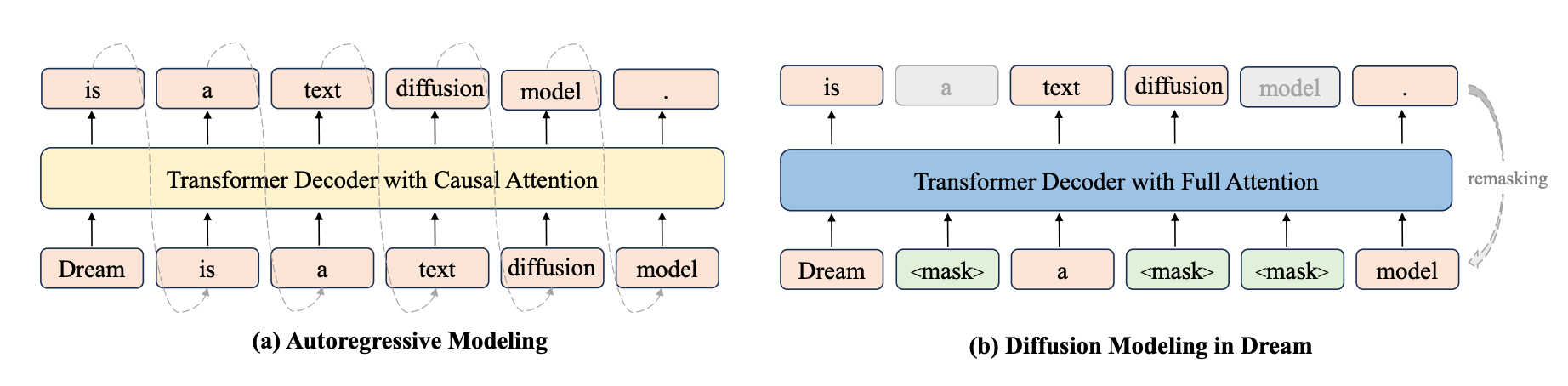
Dream 7B is still trained in a diffusion-style way: we take a clean sentence, add noise by masking some tokens, and train the model to recover the original tokens at the masked positions. The key difference is that we don’t throw away the autoregressive (AR) structure that Qwen2.5 already learned:
In Qwen2.5, the model is trained to look at previous tokens and predict the next one.
When we switch to diffusion, we keep this left-to-right habit instead of forcing the model to learn a new “predict the token at this same position” behavior from scratch.
So internally, Dream still thinks in a “next-token” way, but now it sees a noised, fully visible sentence (both left and right context) and uses that to fill in the masks.
From the outside, you can think of it simply as:
Dream is a diffusion model that predicts masked tokens, but its internal wiring is reused from the original AR model so it doesn’t lose its left-to-right knowledge.
Context-Adaptive Token-Level Noise Rescheduling
In real sentences, not all masked tokens are equally hard to guess. Consider:
[MASK] went to the store because [MASK] was hungry.The first mask has very little context. The second mask is much easier to guess as something like he or she because the sentence already tells us a lot.
Traditional discrete diffusion training does not distinguish these cases very well. It picks one global noise level for the whole sentence, then asks the model to denoise all tokens under that same setting. But learning actually happens token by token, and some tokens may be effectively over-noised or under-noised for their difficulty.
Dream introduces context-adaptive noise rescheduling at the token level:
For each masked token, we estimate how strongly it is supported by its surrounding context.
Easy tokens (with rich context) are treated as if they were in a later denoising step, with less effective noise.
Hard tokens (with weak context) are treated as if they were in an earlier step, with more effective noise.
This aligns the training signal with how much information the model really has for each position, leading to more effective learning across tokens with very different contextual support.
Results: Dream matches or surpasses strong autoregressive models on general, math, and coding benchmarks. It performs particularly well on planning-style tasks (e.g., Sudoku, Countdown) and constraint-satisfaction problems, where iterative refinement is helpful.
Block Diffusion: “Can We Have Both AR and Diffusion?”
Block Diffusion (BD3-LMs) is the most architecturally elegant solution. Instead of choosing between AR and diffusion, it combines them.
The Idea: Divide the sequence into blocks of size B.
Across blocks: Autoregressive factorization
\(p_{\theta}(x) = \prod_{k} p_{\theta}\bigl(x^{(k)} \mid x^{(<k)}\bigr)\)Within each block: Masked diffusion over the B tokens.
Why this is brilliant:
Variable length: Keep generating blocks left-to-right, just like AR. No fixed-length assumption.
KV cache: Cache keys/values across blocks. Each new block only attends to prior blocks, not future ones. This brings back AR’s inference efficiency.
Parallelism: Inside a block, you denoise all B tokens in parallel. You get diffusion’s refinement power locally.
Tunable trade-off: Let L’ be the block size (tokens per block):
If L’ = 1, each “block” is just one token.
The model collapses to a standard autoregressive LM.
If L’ = L, the whole sequence is a single block.
You recover a full-sequence diffusion LM.
For intermediate block sizes (e.g., L’ = 4, 8, 16 in the BD3-LM experiments),
you get a middle ground: some parallel, diffusion-style refinement inside each block but still efficient left-to-right generation across blocks with KV caching.
Results: BD3-LMs achieve state-of-the-art likelihood among discrete diffusion models and close the gap to AR on perplexity benchmarks, while supporting flexible-length generation and fast block-wise caching.
The Hybrid Future: Why AR and Diffusion Work Better Together
Diffusion isn’t replacing autoregressive (AR) models; they’re better together. The most promising systems blend them in three main ways:
1. AR-Initialized Diffusion (Dream, DiffuLLaMA, Mercury)
Start with a standard AR model trained on huge amounts of data. This gives you knowledge and basic reasoning. Then add diffusion training on top. This helps the model plan better, think about the whole picture, and keep its output consistent. You get a model that knows as much as a regular LLM but organizes its answers more carefully.
2. Semi-Autoregressive Hybrid (Block Diffusion, Fast-dLLM v2)
The model generates text in blocks. AR handles the basic structure of what comes first, second, third. Diffusion works inside and across those blocks to refine the details. This keeps the speed and flexibility of AR while improving fluency and consistency.
3. Diffusion as Drafter
This pattern uses one model as a fast drafter and the other as a verifier. The diffusion model can act as the drafter, generating multiple tokens in parallel while the AR model verifies and corrects the sequence.
References
Devlin, J. et al. “BERT: Pre-training of Deep Bidirectional Transformers for Language Understanding.” NAACL 2019.
https://arxiv.org/abs/1810.04805 (arXiv)Berglund, L. et al. “The Reversal Curse: LLMs Trained on ‘A is B’ Fail to Learn ‘B is A’.” ICLR 2024.
https://arxiv.org/abs/2309.12288 (arXiv)
Li, X. L. et al. “Diffusion-LM Improves Controllable Text Generation.” NeurIPS 2022.
https://arxiv.org/abs/2205.14217 (arXiv)Austin, J. et al. “Structured Denoising Diffusion Models in Discrete State-Spaces (D3PM).” NeurIPS 2021.
https://arxiv.org/abs/2107.03006 (arXiv)Gulrajani, I., Hashimoto, T. B. “Likelihood-Based Diffusion Language Models.” NeurIPS 2023.
https://arxiv.org/abs/2305.18619 (arXiv)Sahoo, S. S. et al. “Simple and Effective Masked Diffusion Language Models.” NeurIPS 2024.
https://arxiv.org/abs/2406.07524 (arXiv)
Nie, S. et al. “Large Language Diffusion Models (LLaDA).” 2025.
Paper: https://arxiv.org/abs/2502.09992 (arXiv)
Project page: https://ml-gsai.github.io/LLaDA-demo/ (ml-gsai.github.io)Ye, J. et al. “Dream 7B: Diffusion Large Language Models.” 2025.
Paper (PDF): https://arxiv.org/pdf/2508.15487 (arXiv)
Blog: https://hkunlp.github.io/blog/2025/dream/ (hkunlp.github.io)Arriola, M. et al. “Block Diffusion: Interpolating Between Autoregressive and Diffusion Language Models (BD3-LM).” ICLR 2025.
Paper (PDF): https://arxiv.org/pdf/2503.09573 (arXiv)
Code: https://github.com/kuleshov-group/bd3lms (GitHub)Gong, S. et al. “Scaling Diffusion Language Models via Adaptation from Autoregressive Models (DiffuGPT, DiffuLLaMA).” ICLR 2025.
Paper: https://arxiv.org/abs/2410.17891 (arXiv)
Code: https://github.com/HKUNLP/DiffuLLaMA (GitHub)
About the authors
Aman Gokrani and Ayush Nangia are researchers at Lossfunk